Tutorial: momentum-kick searches (ultraheavy dark matter)

A dedicated walkthrough for impulse ("kick") searches with levitated sensors — the ultraheavy-dark-matter (UHDM) setting where a single DM particle flying past a levitated test mass delivers one measurable momentum transfer. The runnable companion is examples/uhdm_momentum_kicks.py:

python examples/uhdm_momentum_kicks.py

For the generic method see TUTORIAL.md; for the statistics, EXPLANATION.md.

The physics setting

An UHDM particle (say \(m_\text{DM} \sim 10^6\text{–}10^{12}\) GeV) coupled to neutron number through a long-range Yukawa force scatters off a levitated sensor and imparts an impulse. Each candidate event has one measured observable: the momentum transfer \(q\), reconstructed from the sensor's ringdown. The experiment counts kicks above a momentum threshold \(q_\text{th}\) over a livetime \(T_\text{obs}\). (Public references for this class of search: Monteiro et al., arXiv:2007.12067; Amaral et al., arXiv:2409.03814.)

Three facts make this an optimum-interval problem:

1. The signal shape in \(q\) is known per mass. For a massless mediator, integrating the classical Coulomb-like cross section over a Maxwell–Boltzmann halo gives

$\(\frac{dR}{dq} \propto \frac{1}{q^3}\left[e^{-(q/2\mu v_0)^2} - e^{-(v_\text{esc}/v_0)^2}\right], \qquad q \in [q_\text{th},\, 2\mu v_\text{esc}],\)$

with \(\mu \simeq m_\text{DM}\) (the sensor is far heavier). Different masses predict different spectra and kinematic endpoints — exactly like WIMP recoil spectra vs WIMP mass.

1. The normalization is the one unknown. The rate scales as \((\alpha_n N_n)^2\) — the coupling per neutron squared, times the sensor's neutron number squared.

2. The background is real but unmodelable. Seismic/vibrational transients, cryostat events, and cosmic rays produce impulse-like candidates that pile up just above threshold, and none of them can be modeled to subtraction precision. This is the "unknown background" the optimum interval was invented for.

Where the usual method breaks

The standard limit for these searches is: "we observe zero events above \(q_\text{th}\), so we exclude any coupling predicting \(\langle N\rangle \gtrsim 3\)" (95% CL zero-event Poisson).

That is correct — it is the zero-event special case of the optimum interval: with no events, the whole window is one gap, and the 95% optimum-interval limit is \(\mu_\text{UL} = -\ln 0.05 \simeq 3.0\) (the example verifies this numerically). But the rule is brittle: the first candidate that survives your cuts forces a bad choice —

• call it background (indefensible without a background model), or
• take the full Poisson multiplicity hit at every mass, or
• raise \(q_\text{th}\) until zero events remain — a data-driven cut with an uncorrected trials factor, the very bias Yellin's paper opens with.

The optimum interval is the drop-in generalization: it uses the emptiest stretch of the spectrum (chosen and calibrated correctly), so background candidates clustered near threshold barely affect masses whose spectra extend to high \(q\).

The workflow

Step by step from examples/uhdm_momentum_kicks.py:

1. Signal shape → spectrum_cdf. Integrate \(dR/dq\) on a log grid and hand the samples to spectrum_cdf_from_samples, which normalizes the window onto \([0,1]\):

def kick_spectrum_cdf(m_dm):
    q = np.geomspace(Q_TH, q_max(m_dm), 4000)
    pdf = drdq_alpha1(q, m_dm)
    cdf = np.concatenate([[0.0], np.cumsum(0.5 * (pdf[1:] + pdf[:-1]) * np.diff(q))])
    return spectrum_cdf_from_samples(q, cdf / cdf[-1])

2. Per mass, keep only kinematically allowed candidates. A kick with \(q > 2\mu v_\text{esc}\) cannot be signal for that mass, so it drops out of that mass's analysis window:

inside = KICKS[(KICKS > Q_TH) & (KICKS < q_max(m))]

3. Limit on the expected count. One Monte-Carlo calibration table serves every mass (the calibration lives in cumulant space):

table = OptimumIntervalTable(rng=np.random.default_rng(0))
mu_ul = table.upper_limit(inside, confidence=0.95,
                          spectrum_cdf=kick_spectrum_cdf(m), n=4000)

4. Count → coupling. Because the rate is quadratic in the coupling, \(N(\alpha_n) = (\alpha_n N_n)^2\, R(\alpha{=}1)\, T_\text{obs}\), the limit inverts with a square root:

\[\alpha_n^\text{lim} = \frac{1}{N_n} \sqrt{\frac{\mu_\text{UL}}{R(\alpha{=}1)\,T_\text{obs}}}.\]

A 2× stronger \(\mu_\text{UL}\) is therefore \(\sqrt2\) in the coupling.

What the example shows

With five toy candidates — four transients just above an 8.4 TeV threshold plus one outlier at 30 TeV (all fiducial numbers, not a real dataset):

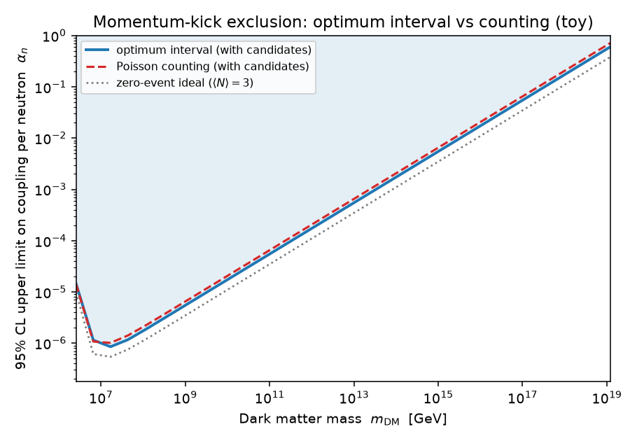
• High mass (all candidates in-window): Poisson counting gives \(\mu_\text{UL} = 10.5\); the optimum interval gives \(\simeq 7.4\) by limiting from the empty stretch between the threshold cluster and the endpoint — ~20% stronger in \(\alpha_n\), with no background model.
• Near threshold (narrow window, events fill it): the optimum interval \(\approx\) Poisson, as it must — when the data look signal-like everywhere, there is no empty region to exploit and no method can do better.
• The gray dotted curve is the zero-event ideal (\(\mu = 3\)): reachable only if the detector stays perfectly quiet. The optimum interval is the principled way to get close to it when it doesn't.

Caveats

• At 95% CL no coupling giving \(\mu < 3.0\) can be excluded (the analog of Yellin's \(\mu < 2.3\) floor at 90%) — the zero-event limit is already optimal.
• The optimum interval is conservative by construction: coverage is at least 95%, never less, whatever the background.
• Finite mediator mass (\(\lambda < \infty\)) changes the shape \(dR/dq\), and makes it depend on the coupling itself, so the single-solve upper_limit no longer applies directly. The worked notebook uhdm_finite_range.ipynb handles that case by scanning the coupling and evaluating the extremeness with the package primitives at each grid point, for the seven planned mediator ranges \(\lambda\) = 2 m down to 0.2 µm in decade steps (sensor radius \(R_\text{eff}\) = 200 µm).
• Likewise the halo model: the example uses the simplified Maxwell–Boltzmann distribution (no Earth motion; \(v_\text{esc}\) enters only as the integration cutoff). Upgrading to the full truncated, boosted distribution is again just a different \(dR/dq\) fed to spectrum_cdf_from_samples.
• All experiment parameters in the example (\(q_\text{th}\), \(N_n\), \(T_\text{obs}\), halo values) are illustrative fiducials — substitute your experiment's.