The Optimum Interval Method, for a Phenomenologist¶
A guide to Yellin's method for setting upper limits in the presence of unknown background — enough to understand it and reimplement it from scratch.
Reference: S. Yellin, "Finding an Upper Limit in the Presence of Unknown
Background", Phys. Rev. D66 (2002) 032005, arXiv:physics/0203002.
Equation and figure numbers below refer to that paper. Code references point at
this repository's src/optimum_interval/.
TL;DR¶
You want a frequentist one-sided upper limit on a signal normalization — for a direct-detection experiment, the WIMP–nucleon cross section \(\sigma\), which fixes the expected number of signal events \(\mu\). Your problem: there may be a background you cannot model or subtract. Any method that needs the likelihood (profile likelihood, Feldman–Cousins, Bayesian posteriors) is stuck, because the likelihood contains the unknown background density.
Yellin's insight: an unknown physical background can only add events. So a region of the observable that is anomalously empty, relative to what the proposed signal predicts, is evidence that the proposed signal is too strong — and no amount of unknown background can rescue it. Turn "the emptiest region is too empty" into a test statistic, calibrate that statistic with a background- free Monte Carlo, and you get a true (if conservative) classical upper limit that (i) needs only the signal shape, (ii) uses no binning, and (iii) is invariant under any reparametrization of the observable.
Two variants: - Maximum gap (\(C_0\)): use the single largest event-free gap. Has a closed-form calibration (Eq. 2) — no Monte Carlo needed. - Optimum interval (\(C_\text{max}\)): generalize "gap with 0 events" to "interval with \(\le n\) events", and let the data pick the most constraining interval. Stronger, but needs Monte Carlo. This is the method the repo's name refers to.
Notation¶
| symbol | meaning |
|---|---|
| \(E\) | the observable measured per event (e.g. nuclear-recoil energy) |
| \(dN/dE\) | expected signal spectrum shape at the proposed \(\sigma\) (known) |
| \(\mu\) | total expected signal events over the analysis range \(=\int dN/dE\,dE\) (unknown, \(\propto\sigma\)) |
| \(\epsilon(E)\) | the cumulant: expected fraction of signal below \(E\) (a CDF, \(\in[0,1]\)) |
| interval size \(x\) | expected number of signal events inside an interval |
| \(n\) | number of observed events inside an interval |
| \(C_0(x,\mu)\) | prob. the maximum gap is smaller than \(x\) (Eq. 2) |
| \(C_n(x,\mu)\) | prob. that all intervals with \(\le n\) events have size \(\le x\) |
| \(C_\text{max}\) | the test statistic: max over intervals of \(C_n(x,\mu)\) |
| \(\bar{C}_\text{max}(C,\mu)\) | value of \(C_\text{max}\) reached with probability \(C\) (the calibration; Fig. 2) |
1. The statistical problem, and why the usual machinery fails¶
Events lie along a one-dimensional observable \(E\). For a proposed cross section \(\sigma\) you know the shape \(dN/dE\) of the signal (astrophysics × form factor × detector response), and \(\mu(\sigma)=\int dN/dE\,dE \propto \sigma\) is the only free normalization. There may additionally be a background whose per-unit-\(E\) rate is non-negative but otherwise unknown and non-subtractable.
Write the likelihood of the observed energies \(\{E_i\}\):
Every likelihood-based method — maximum likelihood, the Feldman–Cousins likelihood-ratio ordering [Phys. Rev. D57 (1998) 3873], a Bayesian posterior — needs the background density \(b(E)\). If you genuinely cannot model \(b(E)\), you cannot write \(\mathcal L\), and all of these are unavailable. The traditional fallback is a single-interval Poisson limit: pick an energy window, count \(N_\text{obs}\), and exclude any \(\mu\) that would give \(>N_\text{obs}\) with probability \(>C\). This works but is badly biased by the choice of window: put the window where noise piles up and your limit inflates; hand-tune the window to the data and you bias low.
The optimum-interval method keeps the good idea (look where the data are empty) but removes the bias by choosing the interval with the data and then correctly accounting for that choice via Monte Carlo. The crucial one-sided logic:
Unknown background is \(\ge 0\), so it can only raise event counts. An interval that contains fewer events than the proposed signal predicts therefore bounds the signal from above, and background cannot invalidate that bound.
This is why the limit is conservative (never under-covers) regardless of the background, and why it uses only the signal shape.
2. The cumulant transform: everything becomes uniform¶
The engine of the method is the probability-integral transform. Define the normalized cumulant
If signal events are drawn from \(dN/dE\), then \(\epsilon(E)\) is uniform on \([0,1]\), whatever the shape of \(dN/dE\). Equivalently, in the unnormalized coordinate \(z(E)=\int_{E_\text{min}}^E dN/dE'\,dE'\) running from \(0\) to \(\mu\), signal events are uniform with unit density, and the total length of the range equals \(\mu\).
Two consequences do all the work:
- Shape independence. After the transform every signal looks the same — a uniform process — so a single Monte Carlo (uniform points) calibrates all spectra. The shape only re-enters through where the observed events land in \(\epsilon\).
- Parameter invariance. The "size" of an interval, \(x=\int_\text{interval} dN/dE\,dE=\Delta z=\mu\,\Delta\epsilon\), is the expected event count in it. It is invariant under any one-to-one change of the observable (\(E\to\) anything monotonic), so the limit does not depend on whether you bin in energy, \(\log\) energy, recoil velocity, ….
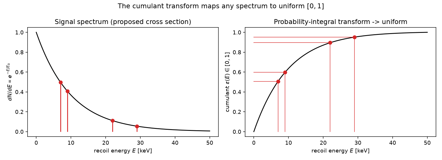
Worked mini-example (this is explanatory_figures() in
reproduce_figures.py; see figures/explain_cumulant_transform.png). Take an
exponential recoil spectrum \(dN/dE\propto e^{-E/E_0}\) with \(E_0=10\) keV on
\([0,50]\) keV, normalized so \(\mu=5\) expected events. Its CDF is
Four toy events at \(E=\{7,9,22,29\}\) keV map to cumulants \(\epsilon\approx\{0.51,0.60,0.90,0.95\}\). Prepend the range boundary \(0\) and append \(1\), giving the point list \(\{0,\,0.51,\,0.60,\,0.90,\,0.95,\,1\}\) on the unit interval — the maximum gap is clearly the empty stretch from \(0\) to \(0.51\). From here on we never need the spectrum again — only this list.
In code: the transform is cumulant_points(events, spectrum_cdf) in
intervals.py, which sorts, applies the CDF, and adds the \(0\) and \(1\)
boundaries.
3. The maximum gap method and its closed form (Eq. 2)¶
The maximum gap is the largest interval between two adjacent events (Fig. 1) — i.e. the widest empty stretch — measured by its size \(x=\int_{E_i}^{E_{i+1}}dN/dE\,dE\) (Eq. 1). If the proposed \(\sigma\) is too big, the expected density is high everywhere and it becomes very unlikely to see such a wide empty gap. Formally, define
A large observed gap gives \(C_0\) near 1. The 90% CL upper limit is the \(\mu\) (hence \(\sigma\)) at which the observed maximum gap \(x_\text{obs}\) satisfies \(C_0(x_\text{obs},\mu)=0.90\).
Yellin derives the closed form (Eq. 2, Appendix A):
Derivation sketch (full version in Appendix A). Let \(P(x;n,\mu)\) be the probability that the maximum gap among \(n\) uniform events on \((0,\mu)\) is \(<x\). Scaling to the unit interval gives \(P(x;n,\mu)=P(x/\mu;n,1)\). A one-step recursion in the number of events,
is solved piecewise to give \(P_m(x;n)=\sum_{k=0}^m(-1)^k\binom{n+1}{k}(1-kx)^n\) (with the analytic-continuation convention for the binomial). Averaging over a Poisson-distributed \(n\) collapses the double sum into Eq. 2.
Numerical note. The factor \(\bigl(1+\tfrac{k}{\mu-kx}\bigr)\) is singular when \(\mu=kx\). Multiplying it in telescopes to the algebraically identical but division-free
which is what analytic.c0(x, mu) evaluates. The series is only well-conditioned
near \(C_0\sim0.9\) (small \(m\)); for \(x\) far below the typical gap (\(m\) huge) the
value underflows to \(0\) and we return \(0\) directly. No Monte Carlo is needed
for the maximum gap, which is why we use \(C_0\) as the ground-truth check on the
simulation (§8, figures/c0_validation.png).
analytic.x0(0.9, mu) inverts this: the gap size at which \(C_0=0.9\).
4. From gaps to optimum intervals: \(C_\text{max}\)¶
When there are enough events that even the largest gap is not very constraining, generalize: instead of intervals with 0 events, consider intervals with \(\le n\) events. Define
\(C_0\) is the maximum-gap case. \(C_n\) increases with \(x\), decreases with \(n\), and (the key property) is independent of the signal shape once \(x\) and \(\mu\) are fixed — again because of the cumulant transform. For \(n\ge1\) it has no simple closed form and is tabulated by Monte Carlo.
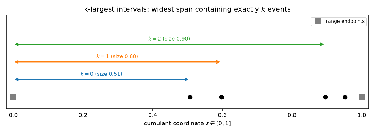
The search is finite. Any interval can be widened until it just touches an event or a range endpoint without changing how many events it contains — which only raises \(x\) and hence \(C_n\). So only intervals delimited by events or by the two endpoints matter: for \(N\) events there are \((N+1)(N+2)/2\) of them.
The test statistic is the most constraining one:
Large \(C_\text{max}\) ⇒ some interval is far emptier than the proposed signal allows ⇒ strong evidence \(\sigma\) is too high. Because \(C_\text{max}\) is itself chosen using the data, we must calibrate it: define \(\bar{C}_\text{max}(C,\mu)\) as the value such that a fraction \(C\) of background-free experiments give \(C_\text{max}<\bar{C}_\text{max}(C,\mu)\). The 90% CL upper limit on \(\sigma\) is where the experiment's \(C_\text{max}\) equals \(\bar{C}_\text{max}(0.9,\mu)\) (Fig. 2). Since real background only inflates counts, it can only lower the observed \(C_\text{max}\), so the limit stays valid (conservative).
4.1 How the code computes \(C_n\) — and why it is exactly Yellin's¶
At first glance the code looks like it computes something simpler than Yellin's \(C_n\). It does not — the two coincide, thanks to a nesting property. Here is the mapping:
- For each \(k\),
k_largest_intervalsreturns the size of the largest interval containing exactly \(k\) events (intervals.py). OptimumIntervalTable.extremeness_of_interval(x, k, mu)returns the empirical CDF of that \(k\)-largest size over background-free trials — the fraction of trials whose \(k\)-largest interval is smaller than \(x\) (montecarlo.py).optimum_interval_statistictakes the max over \(k\) — the code's \(C_\text{max}\).
Why the \(k\)-largest CDF equals \(C_n\). Yellin's \(C_n(x,\mu)\) is the joint statement "all intervals with \(\le n\) events have size \(\le x\)." But within any single realization the \(k\)-largest sizes are strictly nested,
because any interval with \(j\) events can be widened to swallow one more event, producing a strictly larger interval with \(j+1\) events. Hence the largest interval with \(\le n\) events is precisely the \(n\)-largest one, and
So \(C_n(x,\mu)=\Pr[s_n\le x]\) — the plain CDF of the single \(n\)-largest
interval, which is exactly what extremeness_of_interval estimates. The joint
condition collapses to the marginal; there is no approximation. (The one place
this must be handled with care is a trial with fewer than \(n\) events, whose
largest \(\le n\)-event interval is the whole range, size \(1\): such a trial never
counts as "\(s_n<x\)" for \(x<1\), which the code reproduces by keeping it in the
denominator but absent from the \(k\)-reference — see §5.)
Consequently optimum_interval_statistic reproduces Yellin's \(C_\text{max}\) up
to Monte-Carlo estimation noise, and the reproduced \(\bar{C}_\text{max}(0.9,\mu)\)
matches the paper quantitatively (e.g. \(0.976\) at \(\mu=54.5\), §10). The only
methodological simplification is that this code also tabulates the \(n=0\) term by
Monte Carlo instead of using the exact Eq. 2 — noisier for \(n=0\), but the same
statistic. Coverage is validated directly in §10 (out-of-sample exceedance
\(=0.100\)).
5. Building \(\bar{C}_\text{max}\) by Monte Carlo¶
For a fixed \(\mu\), the calibration distribution is built by
OptimumIntervalTable.generate(mu, n) (montecarlo.py):
- Trials.
generate_trials(mu, n): for each of \(n\) trials draw \(N\sim\text{Poisson}(\mu)\), draw \(N\) uniforms on \((0,1)\), and add the range endpoints \(0\) and \(1\). (Endpoints act as interval delimiters, exactly as for real data — this is where "intervals terminated by an endpoint" comes from.) - Inner tables. For each trial compute all \(k\)-largest sizes; collect them
into
itv_sizes[mu][k](per-\(k\) arrays across trials). - Statistic per trial.
opt_itvs[mu][t]= \(C_\text{max}\) of trial \(t\) = \(\max_k\) (empirical CDF of \(\text{size}_k\)). Computed with a vectorizedsearchsortedandnp.maximum.at. - Threshold. \(\bar{C}_\text{max}(C,\mu)\) = the \(C\) quantile of
opt_itvs[mu](bar_c_max).
Four points a reimplementer must get right:
- In-sample calibration. The inner extremeness of a trial is computed against a reference set that includes that same trial. This is a small self-referential bias; using two independent MC samples (one for the inner CDFs, one for the outer) removes it. Negligible at large \(n\) (the out-of-sample coverage check in §10 lands on \(0.100\)).
- Denominator convention — this is correct, don't "fix" it.
extremeness_of_intervaldivides by the total trial count \(n\), even for large \(k\) where fewer trials have a \(k\)-largest interval. This is not a quirk: a trial with fewer than \(k\) events has its largest \(\le k\)-event interval equal to the whole range (size \(1\)), which is never \(< x\) for \(x<1\), so it correctly does not count in the numerator while still belonging in the denominator. Dividing instead by the number of trials that have a \(k\)-interval would bias the estimate of \(C_k\) and break the calibration. - Strict inequalities / discreteness. Extremeness uses strict "\(<\)" in steps of \(1/n\); near the 90th percentile with small \(n\) this granularity matters. The strict "\(<\)" also gives \(C_n(\mu,\mu)=\Pr[\text{>}n\text{ events}]\) at the whole-range interval (Appendix B), which is what keeps \(C_\text{max}\) non-trivial.
- Endpoints on both paths. The Monte-Carlo trials include the \(0\)/\(1\)
endpoints, so real data must too. The original code omitted them on the
real-data path; this repo adds them in
cumulant_points, making the two paths consistent. (This does not affect the Fig. 2 reproduction, which is MC-only.)
6. Getting the upper limit: root finding¶
The limit is the \(\mu\) at which the observed statistic reaches the requested
quantile — i.e. extremeness_of_opt_itv_stat evaluated at the observed
\(C_\text{max}\) equals \(C\):
upper_limit
(montecarlo.py) does a coarse integer scan for the first \(\mu\) where
\(f(\mu)=\text{extremeness}-C\) turns positive, then refines with Brent's method
(scipy.optimize.brenth). Monotonicity — a larger proposed \(\mu\) makes the
observed emptiness look more anomalous, raising \(C_\text{max}\)'s extremeness —
justifies the bracketing scan.
Practical notes / knobs (all exposed as keyword arguments so nothing is a magic
number): mu_scan_start, mu_scan_stop, bracket, xtol, n. Because the
empirical CDF is a step function, Brent on it with xtol=1e-2 is deliberately
crude; for production, precompute \(\bar{C}_\text{max}\) on a \(\mu\) grid and
interpolate (as Yellin's Fortran does) rather than regenerating tables inside the
root find.
7. Reimplement it yourself¶
A self-contained recipe. Each step names the function here that implements it.
- Signal model. From the proposed \(\sigma\) and mass, build \(dN/dE\), its
normalized CDF \(\epsilon(E)\), and \(\mu=\int dN/dE\). (User-supplied
spectrum_cdf.) - Transform the data. \(\epsilon_i=\epsilon(E_i)\); sort; prepend \(0\), append
\(1\). (
cumulant_points.) - \(k\)-largest intervals. For each \(k\), \(\text{size}_k = \max_i (\epsilon_{i+k+1} - \epsilon_i)\).
(
k_largest_intervals.) - Background-only MC at this \(\mu\). Per trial: \(N\sim\text{Poisson}(\mu)\);
\(N\) uniforms; add \(0,1\); sort. (
generate_trials.) - Inner calibration. For each \(k\), empirical CDF of \(\text{size}_k\) over
trials. (
itv_sizes,extremeness_of_interval.) - \(C_\text{max}\) statistic. \(C_\text{max}=\max_k \text{CDF}_k(\text{size}_k)\).
(
optimum_interval_statistic.) - Outer calibration. Distribution of \(C_\text{max}\) over trials;
\(\bar{C}_\text{max}(0.9,\mu)\) = its 90th percentile.
(
opt_itvs,extremeness_of_opt_itv_stat,bar_c_max.) - Limit. Scan / root-find \(\mu\) so the observed
\(C_\text{max}=\bar{C}_\text{max}(0.9,\mu)\). (
upper_limit.) - Max-gap shortcut. For the pure max-gap limit, skip MC and solve
\(C_0(x_\text{obs},\mu)=0.9\) with Eq. 2. (
c0,x0.)
# pseudocode
transform:  u = sort(epsilon(E));  points = [0] + u + [1]
sizes[k]  = max_i (points[i+k+1] - points[i])       for k = 0..len-2
for each candidate mu:
    trials = [ sort([0] + uniform(Poisson(mu)) + [1]) for _ in range(n) ]
    ref[k] = [ kth-largest size of trial for trial in trials ]     # per k
    Cmax_trial = [ max_k  mean(ref[k] < size_k(trial))  for trial in trials ]
    Cmax_obs   = max_k mean(ref[k] < sizes[k])
    extremeness(mu) = mean(Cmax_trial < Cmax_obs)
solve extremeness(mu) = 0.9   ->   mu_upper_limit
8. Peculiarities and sanity checks (Appendix B)¶
- \(\mu<2.3026\) is undefined. With probability \(e^{-\mu}>0.1\) an experiment has zero events, giving the maximal possible \(C_\text{max}\); no threshold puts exactly 90% below it. Hence no cross section with \(\mu<2.3026\) can be excluded at 90% CL. (\(e^{-2.3026}=0.1\).)
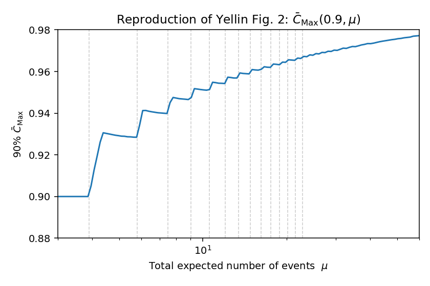
- The curve is not smooth. \(\bar{C}_\text{max}(0.9,\mu)\) jumps upward each time \(\mu\) crosses a threshold where intervals with one more event can first become the maximum. Threshold condition \(C_n(\mu,\mu)=\bar{C}_\text{max}(C,\mu)\) with \(C_n(\mu,\mu)=P(\mu,n+1)=\Pr[{>}n\text{ events in the whole range}]\). Table I of the paper lists them: \(n=0\to2.303\), \(1\to3.890\), \(2\to5.800\), \(3\to7.491\), \(4\to9.059\), …. We overlay these as vertical lines in the Fig. 2 reproduction.
- Flat at 0.90. For \(2.3026<\mu<3.890\) only \(n=0\) can produce \(C_\text{max}\) (intervals with \(\ge 1\) event have \(C_1(\mu,\mu)=\Pr[{>}1\text{ event}]<0.9\) below the \(\mu=3.890\) threshold, so they cannot set the 90th percentile). Then \(\bar{C}_\text{max}(0.9,\mu)=C_0(x_0(0.9,\mu),\mu)=0.9\) exactly — because \(C_0(X,\mu)\) is uniform on \([0,1)\) apart from an atom of mass \(e^{-\mu}\) at \(1\) (the zero-event experiments, whose max gap is the whole range), and that atom sits above the 90th percentile, which therefore falls at \(0.9\). This code reproduces the plateau at \(0.9000\) (measured), since it computes the same \(C_\text{max}\) (§4.1).
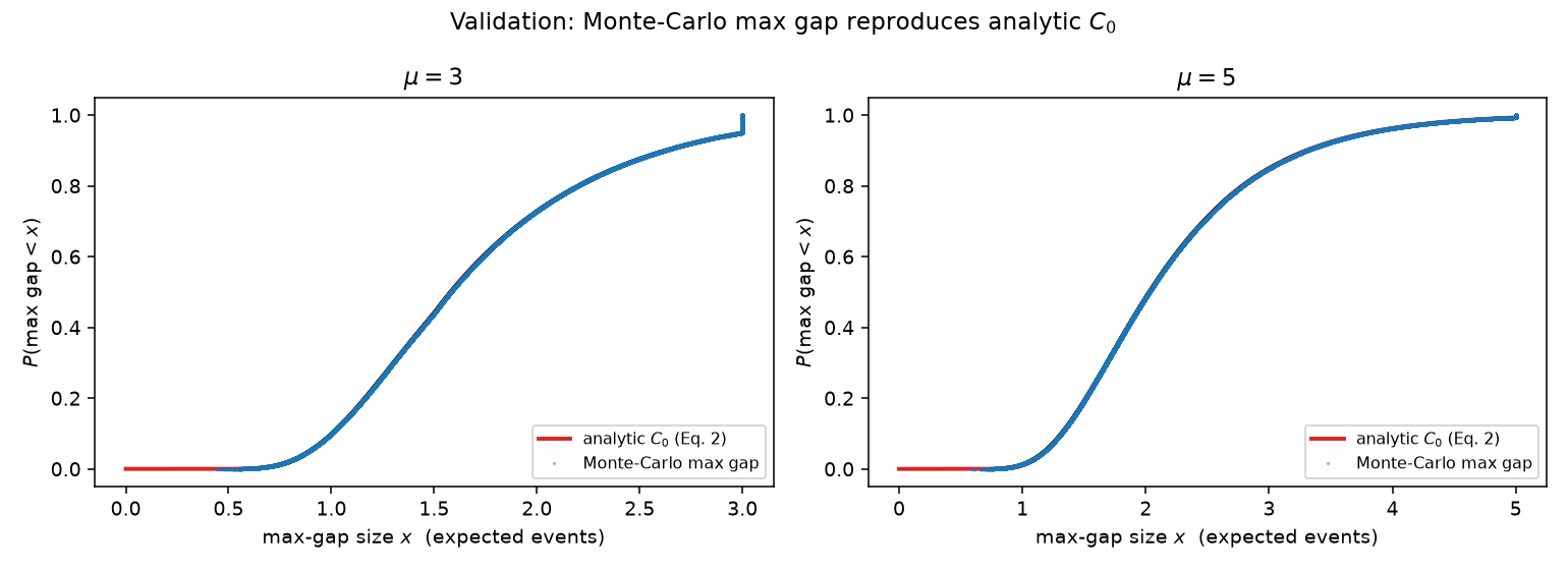
The strongest self-test: the \(k=0\) Monte-Carlo max-gap distribution must equal
the analytic \(C_0\) (Eq. 2). tests/test_montecarlo.py::test_mc_maxgap_matches_analytic_c0
asserts this within \(4/\sqrt n\); figures/c0_validation.png shows it visually.
9. From a limit on \(\mu\) to the cross-section / mass plane¶
For a fixed WIMP mass \(M\) the spectrum shape (and thus \(\epsilon\)) is fixed, and
counts scale linearly with cross section: \(\mu(\sigma,M)=\sigma\,\mu_1(M)\), where
\(\mu_1(M)\) is the expected count per unit \(\sigma\) (astrophysics × form factor ×
exposure). So the upper limit is \(\sigma_\text{UL}(M)=\mu_\text{UL}/\mu_1(M)\).
Walk \(\sigma\) (hence \(\mu\)) up until \(C_\text{max}\) reaches
\(\bar{C}_\text{max}(0.9,\mu)\) (§6), then repeat over a grid of masses to trace the
exclusion curve. Efficiency point: the uniform Monte-Carlo tables are
mass-independent and reusable across all \(M\); only spectrum_cdf changes with
mass.
10. Verification: reproducing the plots¶
Run python reproduce_figures.py --full (see the README). Committed outputs in
figures/:
| figure | what it verifies |
|---|---|
fig02_barCmax_reproduction.png |
Yellin Fig. 2 reproduced: \(\bar{C}_\text{max}(0.9,\mu)\) rises from the ~0.90 plateau to ~0.97 across \(\mu\in[3,100]\) on a log axis, with upward steps aligned to the Table I thresholds (overlaid). |
c0_validation.png |
The \(k=0\) Monte-Carlo max-gap CDF lands on the analytic \(C_0\) (Eq. 2) at \(\mu=3\) and \(\mu=5\) to within Monte-Carlo noise (\(\lesssim0.002\)) — a simulation-free correctness check. |
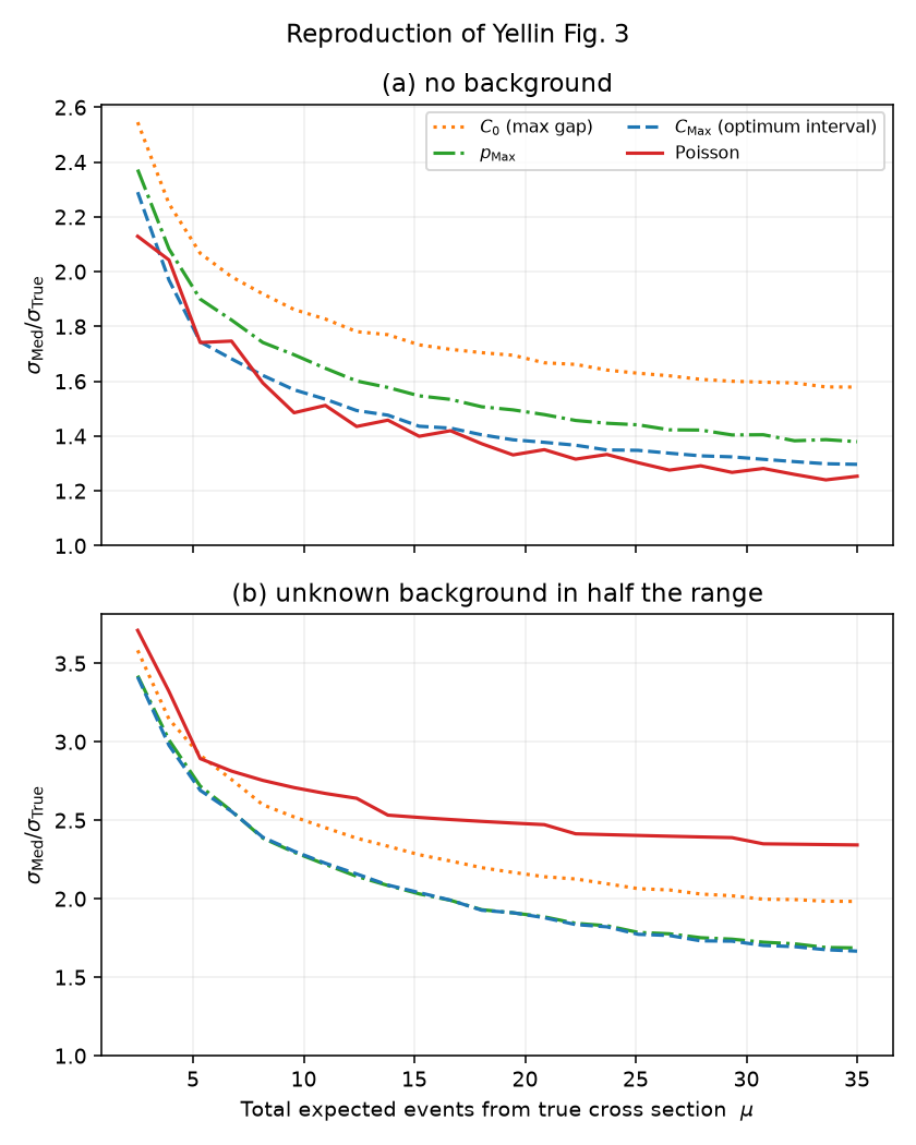
fig03_median_ratio_reproduction.png |
Yellin Fig. 3: median limit ratio \(\sigma_\text{Med}/\sigma_\text{True}\) vs \(\mu\) for all four methods, panels (a) no background / (b) unknown background in half the range. Reproduces the ordering: (a) \(C_\text{max}\!\approx\) Poisson lowest, \(p_\text{max}\) above, \(C_0\) highest; (b) \(C_\text{max}\!\approx p_\text{max}\) lowest, \(C_0\) higher, Poisson worst. (Poisson's paper "jaggedness" from discreteness is smoothed here by the median over a continuous \(\mu\) grid.) |
fig04_mistakes_reproduction.png |
Yellin Fig. 4: fraction of "mistakes" (limit below true) for test (b): \(C_0\) (most) \(> p_\text{max} > C_\text{max}\) (fewest). |
fig05_barpmax_reproduction.png |
Yellin Fig. 5 (bonus, \(p_\text{max}\) method): \(\bar{p}_\text{max}(0.9,\mu)\) vs \(\mu\), with the low-\(\mu\) analytic anchor \(1-e^{-x_0}\) and the \(\mu=5.156\) kink (Table II). |
explain_cumulant_transform.png |
The §2 worked example: an exponential spectrum mapped to uniform. |
explain_klargest_schematic.png |
The §3–4 \(k\)-largest intervals on the unit interval. |
A separate, simulation-based check (not a figure) confirms coverage: at \(\mu_0=15\), fresh out-of-sample background-free experiments exceed \(\bar{C}_\text{max}(0.9,\mu_0)\) a fraction \(0.100\) of the time, as they should for a valid 90% construction.
On the \(p_\text{max}\) low-\(\mu\) anchor. For \(2.3026<\mu<5.156\) only \(n=0\) contributes, so \(\bar{p}_\text{max}(0.9,\mu)=p_0(x_0(0.9,\mu))\). Since the paper defines \(p_n(x)=P(x,n{+}1)=\Pr[{>}n\text{ events}]\), we have \(p_0(x)=1-e^{-x}\), giving \(\bar{p}_\text{max}=1-e^{-x_0(0.9,\mu)}\) — which our Monte Carlo confirms and which reproduces Fig. 5's rise from \(\approx0.9\) toward \(1\). Note the paper's Appendix C prints this closed form as \(e^{-x_0}\); that value is \(\approx0.07\)–\(0.09\) and would sit off the bottom of the plot, so the printed form appears to drop a "\(1-\)".
This covers all five figures of the paper (Fig. 1 is a schematic, previewed by
the two explain_* figures; Figs. 2–5 are reproduced from data). --full
regenerates everything; Figs. 3 & 4 dominate the runtime (a large
experiment-comparison Monte Carlo), so --only compare runs just those.
Each figure records the random seed and Monte-Carlo sample size. Running the
script also writes *_side_by_side.png for each paper figure, placing our
reproduction next to the original panel (extracted read-only from
arXiv-physics0203002v2.tar.gz); those are kept out of version control because
they embed the copyrighted paper figures.
11. Code map¶
| module | contents |
|---|---|
optimum_interval/intervals.py |
k_largest_intervals, cumulant_points — pure interval geometry |
optimum_interval/analytic.py |
c0 (Eq. 2), x0, poisson_upper_limit, max_gap_upper_limit |
optimum_interval/montecarlo.py |
OptimumIntervalTable — MC tables, bar_c_max, upper_limit, persistence |
optimum_interval/spectra.py |
spectrum_cdf_from_pdf, spectrum_cdf_from_samples |
optimum_interval/comparison.py |
ComparisonEngine — fast per-experiment limits (Figs. 3–4) |
optimum_interval/plotting.py |
bar_c_max_curve, plot_bar_c_max — Fig. 2 |
reproduce_figures.py |
regenerate every figure above |
tests/ |
unit tests incl. the MC-vs-\(C_0\) validation |